$T\mathcal{M}$

How many connectives do we actually need?

In classical logic there are several logical connectives, that is the building blocks of terms that connect simpler terms together. The most prominent examples are $\land$, and, and $\lor$, or, which behave in the obvious way. Then a few more are named, negation, $\neg$, which is true whenever it operates on a falsehood. Implication $\rightarrow$, which is probably the first logical operation that is not obvious. In classical logic it abbreviates $A\rightarrow B \equiv \neg A \lor B$ which is somewhat more expansive than we would expect, after all that I am writing this while it is not raining does not obviously imply that it is not raining because I'm writing. However it implies that we can conclude $B$ whenever we observe $A$. Then we can of course introduce additional symbols like equivalence $\leftrightarrow$. Now the question is, how many of these do we actually need and just looking at truth tables, there are $2^4 = 16$ possible 2-ary functions in bivalent logic and inspecting a truth table, two operations should be enough to generate them. For example one rotation and toggling a specific place should suffice, since we can rotate a toggled bit to it's desired place. For the logical connectives doing the same kind of analysis we will need negation, and one of the others to have all sixteen possibilities.

We can express

$$ A\lor B \equiv \neg\left(\neg A \land \neg B\right) $$

that is $A$ or $B$ is the same as not $A$ and $B$ being false. Conversely we have

$$ A\land B \equiv \neg \left( \neg A \lor \neg B\right) $$

that is, $\land$ is true if neither $A$ nor $B$ are false. This implies that we can do without one of these. The third one, $\rightarrow$, is given above already as

$$ A\rightarrow B \equiv \neg A \lor B $$

and is true whenever observing A is sufficient to conclude B. Implication has an obvious bidirectional cousin, equivalence

$$ A\leftrightarrow B \equiv \left(A\rightarrow B \right) \land \left(B\leftarrow A\right)\\ \equiv \left( \neg A \land \neg B\right) \lor \left(A \land B \right) $$ which implies that either both are true or neither. Here we see they can also be reduced to either $\land$ or $\lor$ and negation. It is however not possible to express negation in terms of the other,

$$ \neg A \equiv ? $$

We could introduce another symbol $\bot$ that always evaluates as false. Then we have

$$\neg A \equiv A\rightarrow \bot \\\equiv \neg A \lor \bot \\\equiv \neg A, $$

but that just introduces another irreducible symbol.

To see that implication can not be expressed in terms of the other, consider the case where $A$ is true, then $A\land A$, $A\lor A$ and $A \rightarrow A$ are true and to build more complex ones we have to connect simpler terms with connectives, but these simpler terms are already true and we will never get one that evaluates to falsehood.

Some fun with definitions of derivatives

The easiest to interpret definition of an derivative $f'$ of an function $f: \mathbb{R}\to\mathbb{R}$ at a point $x_0$ is

$$ f(x)=f(x_0)+ f'(x_0) (x-x_0) + \varphi( x-x_0) $$

such that $\lim_{x\rightarrow x_0} \varphi(x-x_0)/ ||x-x_0||=0$. In particular the definition tells us, that derivatives are a way to approximate functions by linear functions.

More generally the idea, that we can approximate functions by polynomials, is known as Taylor's theorem. In the case of an analytic function $f(x)=\sum_{k=0}^{\infty} a_{k}x^{k}$, we have

$$ \frac{1}{m!} \frac{\partial^m}{\partial x^m} f(0) = a_m $$

and consequently the Taylor expansion up to second order around a point $x_0$

$$ f(x)\approx f(x_0) + f'(x_0) (x-x_0) + 1/2 f''(x_0) x^2 + \mathcal{O}(x^3). $$

We can then argue that the analytic functions are dense in the space of functions to gain a very useful approximation technique from this.

Until yesterday I believed that one could also prove the second function directly from the first definition. However, something interesting happens, let $\varphi$ the error term from the definition, $\varphi_2$ the error term of the error term, and assume $\varphi$ is differentiable:

$$ \varphi(x)=\varphi(x_0)+\varphi'(x_0) (x-x_0) + \varphi_2 (x-x_0)\\ = -f''(x_0) (x-x_0)^2 + \varphi_2 (x-x_0) $$

and following directly

$$ f(x)=f(x_0) + f'(x_0) (x-x_0) - f''(x_0) (x-x_0)^2 + \varphi_2 (x-x_0) $$

which when we compare that with the second order Taylor expansion, we find that

$$ f(x)-\varphi_2 (x-x_0) =\left[f(x_0) + f'(x_0) (x-x_0) + 1/2 f''(x_0) x^2\right]\\ -\frac{3}{2} f''(x_0) (x-x_0)^2 \sim \mathcal{O}(x^2) $$

where the square brackets delimit the Taylor expansion. So $\varphi_2$ is only the right function up to second order (which is precisely the order we need for the definition of the derivative), and therefore we can not get Taylor approximation beyond first order from this definition directly. (It is of course still possible, we just need a better characterization of $\varphi_2$ than we get from the definition.)

A graphical proof of the "Binomische Formeln"

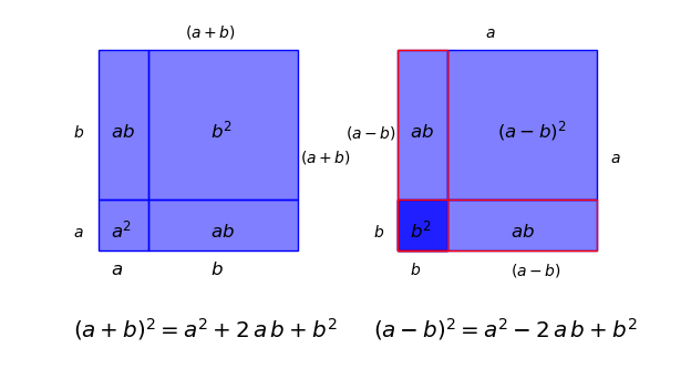
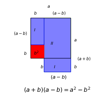
A quick geometric proof of the three formulas $(a\pm b)^2=a^2 \pm 2ab + b^2$ and $(a+b)(a-b)=a^2+b^2$. These three can of course easily be proven by algebraic means, but it is nice to view them in a geometric context. As an aside on mathematical education, the three formulas are a set piece of high school education in Germany under the name "Binomische Formeln," but it appears that they do not have a similar status internationally.

The first two

The proof is simple, for the first "Binomische Formel" $(a+b)^2=a^2+2\,a\,b+b^2$ on the left hand side, we see directly that the square with sides of length $(a+b)$ is composed of a square with side $a$, one with side $b$ and two rectangles, each with one side $a$ and the other $b$ and adding together areas of the four rectangles gives us directly the result.

For the second one on the right, we have a square with side length $(a-b)$, the upper right square. To get from a square with sides $a$ to the one with sides $(a-b)$, we have to subtract the red rectangles, with sides $a$ and $b$, but then we have subtracted the dark blue square with sides $b$ in the lower left corner twice, and therefore we have to add it back.

Third square formula

The third Binomische Formel is $(a+b)(a-b)=a^2-b^2$ and the geometric proof is slightly less straight forward. We start with the rectangle $II$, with the sides $(a+b)$ and $(a-b)$ and try to construct the square with sides $a$, the black outline. For that we note first, that the rectangle $II$ decomposes into two parts, one the rectangle with sides $a$ and $(a-b)$ and second the rectangle $I$ at the bottom with sides $b$ and $(a-b)$. Then we move $I$ over to the left side and the missing piece is the square with side length $b$, shown in red.

A note on Bayes' theorem

Thomas Kuhn discussed the notion of paradigms as things that every expert in a field assumes to be true. He then proceeded to study the overturning of these paradigms, scientific revolutions. An example of a paradigm would be the believe of 19th century physicists that every wave needs a medium, which was the key assumption of the ether theory. At the time this was a reasonable believe, every wave studied in detail so far had a medium, air for sound, water for tidal waves and perhaps ropes for demonstration experiments, but light was different. Or perhaps not, it does not take too much redefinition to claim that an unexcited electromagnetic field constitutes a medium. It would certainly not be the medium 19th century physicists had in mind, but with that redefinition we change the claim "19th century physicists were mistaken about the existence of a medium." to "19th century physicists were mistaken about the nature of a medium."

Interestingly a similar thing happens with Bayes' theorem: Let $(X, \mu)$ be a measurable space, $G \subset X$ a subset with finite measure and $A, B \subset G$. Then we can interpret $P(A)=\frac{\mu(A)}{\mu(G)}$ as a probability measure on $G$ and specifically

$$ P(A)=\frac{\mu(A)}{\mu(G)} =\frac{\mu(A\cap G)}{\mu(G)} = P(A|G). $$

Let now $F\subset X$, $\mu(F)$ finite and $A\subset F$. Then

$$ P(B|A)=\frac{P(A\cap B)}{P(A)}\frac{P(B)}{P(B)}\\ =\frac{\mu(A\cap B)}{\mu(A)} \frac{\mu(B)}{\mu(G)} \frac{\mu(G)}{\mu(B)} \left(\frac{\mu(F)}{\mu(F)}\right)^2\\ =P(A|B)\frac{\mu(A)}{\mu(B)} \frac{\mu(F)}{\mu(F)}\\ = P(A|B)\frac{\tilde{P}(B)}{P(A|F)} $$ with $\tilde{P}(B)=\mu(B)/\mu(F)$, for which $\tilde{P}(B)=P(B)$ if $B\subset F$.

This is concerning for two reasons, first there is no relationship between $B$ and $F$. So in case of 'obviously' $F$, one assumes that $B=B\cap F$ and therefore assumes the standard form of Bayes' theorem. On the other hand, even if $B\subset F$, we can not choose between $F$ and $G$. This is the case with the difference between existence and nature of a medium above, it seems that there are interpretive systems that are too strong to be empirically accessible.

The Persian King of King Xerxes had the Hellespont whipped and cursed, after a bridge collapsed. Obviously ridiculous, but the second bridge did hold.

I am not entirely sure, what to make of these. Probably the most conservative interpretation is, a model does not necessarily hold at points were it was not tested. A bit more speculative, we can add believes as long as they do not interfere (too much) with the actual workings of reality.

A proof of Bayes' theorem

A useful way to think about probabilities is as a formalization of Venn Diagrams on measureable spaces. Here I illustrate this point with a proof of Bayes' theorem.

A measurable space is a set $X$ equiped with a measure $\mu$, that is a function from the power set of $X$ to the reals,

$$ \mu : P(X) \rightarrow \mathbb{R} \\ $$

such that

1) It is non-negative $\mu(A) \ge 0$ for all subsets $A\in P(X)$

2) The measure of the empty set vanishes: $\mu(\emptyset)=0$

3) Countable additive, for all countable collections $\lbrace A_{i\in I} \rbrace$ of pairwise disjoint sets

$$ \mu\left(\bigcup\limits_{i\in I} A_i\right) = \sum_{i\in I} \mu(A_i) $$

This definition basically abstracts the notion of an area, an area is never negative, zero only for lower dimensional objects, that is points, lines and the empty set, and if I take two non overlaping shapes, such as one table and another table, then I can add the areas. Note that there can be sets that have a measure of $0$, but are not empty.

As an excercise, one can proof directly that

$$ \mu(A\cup B)=\mu(A)+\mu(B)-\mu(A\cap B) $$

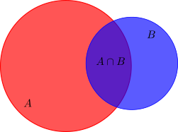
by considering the disjoint sets $A\setminus B$, $B\setminus A$ and $A\cap B$ and noticing that $A\cap B$ is counted twice. Compare this on the Venn diagram below.

We need one extra ingredient for probabilities, the entire set should have measure $\mu(X)=1$, which we can always archive by using $P(A)=\frac{\mu(A)}{\mu(X)}$, if the measure of the entire space is finite. (We can directly check that for such an metric space the Kolmogorov axioms of probability theory hold, and vice versa.)

To gain some intuition, imagine a barn with a target attached. When one throws a dart at the barn the probability to hit the target is $\mu(target)/\mu(barn)$, at least assuming that the dart hits the barn. This motivates the notion of conditional probability. A conditional probability means, that we already know that we hit the barn, what is the probability that we hit the target? Or formally $$ P(A|B)=\frac{P(A\cap B)}{P(B)} $$

which basically states, that if we already know that an event $B$ happens, for example the dart hits the barn, what is now the probability that also $A$ happens. In the illustration above, we already know, that we are in the blue disk and we wonder about the probability, that we hit the shaded area $A\cap B$. More abstractly, we restrict our measurable space from $X$ to $A \subset X$, and the measure to the powerset of $A$.

With this we can now proof Bayes' theorem, for two not impossible events $P(A)\neq 0$, $P(B)\neq 0$ we have the conditional probabilities $$ P(A|B)=\frac{P(A\cap B)}{P(B)} $$ $$ P(B|A)=\frac{P(B\cap A)}{P(A)} $$ And eleminating $P(A\cap B)$ we get the famous formula $$ P(A|B)=\frac{P(B|A)}{P(B)}P(A) $$ which in words say, that the probability that $A$ happens, if we already know that $B$ happens, is the same as the probability that $B$ happens, if we already know that $A$ happens times the ratio of the probabilities $A$ and $B$.

In Bayesian interpretation of probability one considers the probability of an hypothesis $H$ as being true as $P(H)$, then we can use Bayes' theorem to incorporate new information into the hypothesis by using $$ P(H|E)=\frac{P(E|H)}{P(E)} P(H) $$ where $P(H)$ is the probability that the hypothesis is true, $P(E|H)$ is the probability of $E$ given $H$ and $P(E)$ is the overall probability of $E$. The trick here is, that the right hand side is all known information and we can calculate the left hand side. In particular $P(E|H)$ can be calculated from the hypothesis theoretically, since it assumes that the hypothesis is true.

n Times differential functions

Most easy examples of functions are $\mathscr{C}^\infty$, that is they are infinitely often differentiable, like $\sin$ or $\exp$ or polynomials. A rather cute, if trivial, construction of functions that are not is the anti-derivative of the absolute value $|x|$.

$$ \int_0^{x} |\tilde{x}|\,d\tilde{x} = \begin{cases} -\frac{1}{2} x^2 & \text{if $x < 0$} \\ \frac{1}{2} x^2 & \text{if $x \geq 0$} \end{cases} $$

and generalizing to functions $f_n \in \mathscr{C}^n$ but not in $\mathscr{C}^{n+1}$ is

$$ f_n = \begin{cases} - x^n & \text{if $x<0$} \\ x^n & \text{if $x \geq 0$} \end{cases} $$

IOCC 1987 korn.c Analysis

David Korns's 1987 entry to the International Obscufated C Contest (IOCC) is one of the most baffling one liners I have ever encountered. It simply reads

    main() { printf(&unix["\021%six\012\0"],(unix)["have"]+"fun"-0x60);}

and obiviously just outputs unix when compiled on a Linux system. The first thing to analyse something like this is to run it through the preprocessor (and hope that it gets more readable for a change). So after gcc -E the single line from the main function becomes:

printf(&1["\021%six\012\0"],(1)["have"]+"fun"-0x60);

which at least tells us, that unix is a defined in the preprocessor, which actually violates the standard since preprocessor constants should start with two underscores and is switched off if a ansi standard ist explicitly given, like -std=c99. As an aside gcc can be coerced into giving all macros defined by default with

gcc -dM -E  -x c /dev/null

The next thing to clean up is the use of a[b] == b[a] in C, so unix["some string"] is actually the same as "some string"[1] or 'o' and the operator & then effectivly chops off the 's'. Therefore the format string evaluates to (writing type explicitly):

char* f="%six\n" //String literals are automatically null terminated.

The second part, which gets into the output of %s is similarly obscufated. In particular (unix)["have"] == 'a'. It uses one additional trick, (int)'a' is 97 or 0x61, so that the types are char + char* + int and Korn sneaked some pointer arithmetic into the program. So

char* s="fun" + (0x61 - 0x60) // s is "un"

and we end up with the cleaned code of

1
2
3
4
5
6

#include "stdio.h"

int main(){
   printf("%six\n", "fun" + 'a' - 0x60);
   return 0;
}

where the printf is basically

printf("%six\n", "un");