A proof of Bayes' theorem
A useful way to think about probabilities is as a formalization of Venn Diagrams on measureable spaces. Here I illustrate this point with a proof of Bayes' theorem.
A measurable space is a set $X$ equiped with a measure $\mu$, that is a function from the power set of $X$ to the reals,
$$ \mu : P(X) \rightarrow \mathbb{R} \\ $$
such that
1) It is non-negative $\mu(A) \ge 0$ for all subsets $A\in P(X)$
2) The measure of the empty set vanishes: $\mu(\emptyset)=0$
3) Countable additive, for all countable collections $\lbrace A_{i\in I} \rbrace$ of pairwise disjoint sets
$$ \mu\left(\bigcup\limits_{i\in I} A_i\right) = \sum_{i\in I} \mu(A_i) $$
This definition basically abstracts the notion of an area, an area is never negative, zero only for lower dimensional objects, that is points, lines and the empty set, and if I take two non overlaping shapes, such as one table and another table, then I can add the areas. Note that there can be sets that have a measure of $0$, but are not empty.
As an excercise, one can proof directly that
$$ \mu(A\cup B)=\mu(A)+\mu(B)-\mu(A\cap B) $$
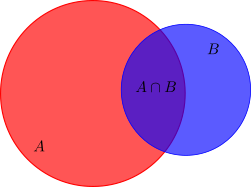
by considering the disjoint sets $A\setminus B$, $B\setminus A$ and $A\cap B$ and noticing that $A\cap B$ is counted twice. Compare this on the Venn diagram below.
We need one extra ingredient for probabilities, the entire set should have measure $\mu(X)=1$, which we can always archive by using $P(A)=\frac{\mu(A)}{\mu(X)}$, if the measure of the entire space is finite. (We can directly check that for such an metric space the Kolmogorov axioms of probability theory hold, and vice versa.)
To gain some intuition, imagine a barn with a target attached. When one throws a dart at the barn the probability to hit the target is $\mu(target)/\mu(barn)$, at least assuming that the dart hits the barn. This motivates the notion of conditional probability. A conditional probability means, that we already know that we hit the barn, what is the probability that we hit the target? Or formally $$ P(A|B)=\frac{P(A\cap B)}{P(B)} $$
which basically states, that if we already know that an event $B$ happens, for example the dart hits the barn, what is now the probability that also $A$ happens. In the illustration above, we already know, that we are in the blue disk and we wonder about the probability, that we hit the shaded area $A\cap B$. More abstractly, we restrict our measurable space from $X$ to $A \subset X$, and the measure to the powerset of $A$.
With this we can now proof Bayes' theorem, for two not impossible events $P(A)\neq 0$, $P(B)\neq 0$ we have the conditional probabilities $$ P(A|B)=\frac{P(A\cap B)}{P(B)} $$ $$ P(B|A)=\frac{P(B\cap A)}{P(A)} $$ And eleminating $P(A\cap B)$ we get the famous formula $$ P(A|B)=\frac{P(B|A)}{P(B)}P(A) $$ which in words say, that the probability that $A$ happens, if we already know that $B$ happens, is the same as the probability that $B$ happens, if we already know that $A$ happens times the ratio of the probabilities $A$ and $B$.
In Bayesian interpretation of probability one considers the probability of an hypothesis $H$ as being true as $P(H)$, then we can use Bayes' theorem to incorporate new information into the hypothesis by using $$ P(H|E)=\frac{P(E|H)}{P(E)} P(H) $$ where $P(H)$ is the probability that the hypothesis is true, $P(E|H)$ is the probability of $E$ given $H$ and $P(E)$ is the overall probability of $E$. The trick here is, that the right hand side is all known information and we can calculate the left hand side. In particular $P(E|H)$ can be calculated from the hypothesis theoretically, since it assumes that the hypothesis is true.